Darwinbots3/Physics

Basic concepts

Forces' linear affects

Any force acting on a body, at any point on a body, applies the same change in acceleration to the body's center of mass. Consider the diagram below:

__________
|        |
|        |  
|   X    |  <--- $\vec{Force_1}$
|        |
|________|  <--- $\vec{Force_2}$

 Diagram 1 

Where X is the center of mass for the body. $\vec{Force_1}$ is exactly centered, so it produces no torque. The change in acceleration of the body's center of mass is given by 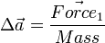$\Delta \vec{a} = \frac{\vec{Force_1}}{Mass}$.

Let $\vec{Force_2}$ have the same magnitude and direction as $\vec{Force_1}$. However it's applying its force at a different point on the body, and will produce torque. Even though it's off center, the change in acceleration for the body's center of mass is still $\Delta \vec{a} = \frac{\vec{Force_1}}{Mass}$.

Forces' angular affects

Consider Diagram 1 again. $\vec{Force_1}$ will not produce any change in angular acceleration for the body, because it is centered. $\vec{Force_2}$ will produce change in angular acceleration, because it is off center. In general, the torque ($\tau$) produced by a force is given by:

$\tau = \vec{F} \cdot \vec{r_{\perp}^{P}}$

And the change in angular acceleration is given by:

$\Delta \alpha = \frac{\tau}{I}$

Where:

• $\tau$ is the scalar torque term.
• $\vec{F}$ is the vector Force term.
• $\vec{r_{\perp}^{P}}$ is the vector perpendicular to the vector from the body's origin to the place $\vec{F}$ is acting on the body.
• $\alpha$ is the scalar angular acceleration
• $I$ is the body's scalar moment of inertertia.

Simple collision

__________      __
|        |     /  |
|        | ___/   |
|   X    |P___  Y |
|        |    \   |
|________|     \__|
 
 Diagram 2 

Consider a collision between two bodies: body X and body Y. They collide at point P. We assume that the collision takes 0 time. That is, the bodies "instantly" resolve their collision.

The change in angular and linear velocity for body X is given by:

$\Delta\vec{v} = \frac{j_0 \cdot \vec{n}}{m_X}$

$\Delta\omega = j_0 * \frac{\vec{r_{\perp}^{XP}} \cdot \vec{n}}{I_X}$

where:

• $\Delta\vec{v}$ is the change in linear velocity.
• $\Delta\omega$ is the change in angular velocity.
• $j_0$ is the scalar impulse term applied to the body at point P to correct its velocity from the collision.
• $m_X$ is the scalar mass for the body.
• $I_X$ is the scalar moment of inertia for the body.
• $n$ is a vector representing the "normal" to the colision. In the case of the vertex-on-edge collision in Diagram 2, n would probably be $<1, 0>$
• $\vec{r_{\perp}^{XP}}$ is the vector perpendicular to the vector from the center of mass of body X to the collision point P.

Body Y likewise, but the changes are opposite in sign (equal and opposite reaction).

We can define a relationship between the velocities before and after the collision using the coefficient of restitution. Which is basically a fractional scalar value between 0 (for inelastic collisions) and 1 (for perfectly elastic collisions).

$v_{XPf} - v_{YPf} = -(1 + \epsilon) * (v_{XPi} - v_{YPi})$

where:

• $v_{XPf}, v_{YPf}$ are the final velocities of bodies X and Y at point P.
• $\epsilon$ is the coefficient of restitution for the equation
• $v_{XPi}, v_{YPi}$ are the initial velocities of bodies X and Y at point P.

To find the velocity of a body at a given point, use the formula:

$v_P = v + \omega * r^P_\perp$

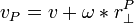
where:

• $v_P$ is the velocity at a certain point on the body.
• $\omega$ is the body's angular velocity.
• $r^P_\perp$ is the vector perpindicular to the vector from the body's center of mass to point P.

Using all of the equations above, we can find $j_0$ by the following algorithm:

suppose we are supplied with:
  a contact point P
  a collision normal n
  two bodies in collision, bodyX and bodyY
  a coefficient of restitution e

Vector VelocityAtPoint(Body body, Vector point)
{
  return body.Velocity + body.AngularVelocity * (point - body.Position);
}

Scalar ResistanceFromBody(Body body, Vector point, Vector n)
{
  Vector rPerp = (point - body.Position).Perp();
  Scalar a = n.LengthSquared() * body.InverseMass; // The resistance to linear acceleration
  Scalar q = Squared(rPerp.DotProduct(n)) * body.InverseMomentOfInertia; // The resistance to angular acceleration
  
  return a + q;
}

Scalar vXP = VelocityAtPoint(bodyX, P);
Scalar vYP = VelocityAtPoint(bodyY, P);

Scalar b = -(1 + e) * (vXP - vYP).DotProduct(n);

Vector rXPNorm = (point - bodyX.Position).Perp();
Vector rYPNorm = (point - bodyY.Position).Perp();

Scalar resistanceX = ResistanceFromBody(bodyX, P, n);
Scalar resistanceY = -ResistanceFromBody(bodyY, P, n); //equal but opposite

Scalar j0 = b / (resistanceX - resistanceY);

return j0;

Multiple collisions

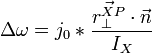
Consider the case of collisions between N bodies simultaneously. We can expand from the last section to handle N contact points. The change in linear and angular velocity of a body is described by the equation:

Failed to parse (unknown function "\Large"): \Delta\vec{v} = \Large{\frac{\sum_{i=0}^{N-1} j_i \cdot \vec{n}}{m}}

Failed to parse (unknown function "\Large"): \Delta\omega = \Large{\frac{\sum_{i=0}^{N-1} j_i \cdot \vec{r_{\perp}^{Pi}} \cdot \vec{n}}{I}}

where:

• $j_i$ is 0 if that contact point isn't part of that body's collision.

We can now form N equations (one for each collision), and solve for N unknowns (each collision impulse $j_i$).

The equation for collision $i$ is given by:

Failed to parse (unknown function "\large"): \large{V_{BPi} + V_{APi} = b_i}

Failed to parse (unknown function "\large"): \large{V_{XPi} = \sum_{k=0}^{k=N-1} (aX_k + qX_k)} \cdot j_k

Failed to parse (unknown function "\large"): \large{aX_k = \frac{\vec{n_i} \cdot \vec{n_k}}{m_X}}

Failed to parse (unknown function "\large"): \large{qX_k = \frac{ (\vec{r^{XPi}_\perp} \cdot \vec{n_i}) \cdot (\vec{r^{XPk}_\perp} \cdot \vec{n_k})}{I_X}}

Failed to parse (unknown function "\large"): \large{b_i = -(1 + \epsilon) ((V_{BP} - V_{AP}) \cdot n_i)}

Failed to parse (unknown function "\large"): \large{V_{XP} = V_X + \omega_X \cdot r^{XP}_\perp}

All terms in the above quantities are known at the beginning of the collision except for $j_i$. So we can represent the system of equation as:

Failed to parse (unknown function "\large"): \large{\mathbf{A} \mathbf{j} = \mathbf{b} }

For an example, suppose that there are 4 collisions. One between body A and body B (collision 0), two between body B and body C (collision 1 and 2), and one between body C and body D (collision 3). If we take the equation for $V_{XPi}$ above, are replace $j_k$ with commas, we can form the system of equations into a matrix:

Failed to parse (unknown function "\large"): \large{ \begin{bmatrix} V_{BP0} - V_{AP0} \\ V_{CP1} - V_{BP1} \\ V_{CP2} - V_{BP2} \\ V_{DP3} - V_{CP3} \\ \end{bmatrix} \begin{bmatrix} j_0 \\ j_1 \\ j_2 \\ j_3 \\ \end{bmatrix} = \begin{bmatrix} b_0 \\ b_1 \\ b_2 \\ b_3 \\ \end{bmatrix} }

Which can then be solved in $O(N^3)$.

Collision detection

Consider the case where all objects in the world are static (not moving). Suppose we want to find a list of bodies which might be colliding. This list might have false positives, but it's much cheaper than the complete collision test. Finding this list of maybe collisions is called broad phase collision detection. The complete collision test where the possibility of false positives and false negatives is eliminated is called narrow phase collision detection.

Broad phase collision detection

This is a mostly comprehensive list of methods for broad phase collision detection:

Naive

The naive broad phase algorithm is just to assume that all bodies might be colliding with each other. The first body is tested against the second, third, fourth, ... nth. The second body is tested against the third, fourth, ... nth. For a total of $\frac{n^2}{2}$ narrow phase collision checks.

The primary advantage to this method is its simplicity to implement and no memory overhead. The downside is that the operation is $O(n^2)$, which makes anything more than about 1000 bodies too slow.

Uniform grid

A uniform grid (also sometimes called a spatial hash) divides the universe into a regular grid of boxes, like a chess board. Each grid square has a list of bodies which are at least partially inside that grid square.

If there are more bodies than grid squares:

For each grid square
  For each pair of bodies in that grid square
    Pass that pair on to narrow phase collision detection

(Watch out for colliding the same pair more than once).

If there are more grid squares than bodies:

 For each body
   For each grid square that body overlaps
     For each otherBody in the current gridSquare
       Pass this body and otherBody on to narrow phase

(Again watch out for colliding the same pair more than once. If each body has a unique serial number, you can just test that the serial number for this body is < the serial number for otherBody).

Worst case performance is still $O(n^2)$ in the case where all bodies are in the same grid square. Average case performance is $O(n)$. It's important to choose an appropriate size for the grid squares. Too large and it's too permissive about passing collisions on to narrow phase. Too small and it starts to waste lots of memory. It also works best when the bodies are all approximately the same size.

Sources: 1 2

Hierarchical grid

An extension of uniform grids from above. A grid size is chosen to be as small as possible without burning too much memory. Above this is constructed a larger grid such that four of the smaller grid squares fit in one of these larger grid squares. This continues recursively up to the very top level. Bodies are placed on the smallest grid level such that they take up only 4 or fewer grid squares.

The primary advantage over uniform grids is a better handling of large bodies. Worst case performance is still $O(n^2)$, though it becomes harder to reach worst case. Average case is still $O(n)$.

Linked list sort

By using the separating axis theorem, we know that a necessary (but not sufficient) effect of two bodies colliding is that their projections onto an arbitrary axis also collide. If we project all bodies on to arbitrary axes, and then sort the result in a linked list, it becomes an $O(n)$ operation to find possible collision pairs. Adding axis allows the test to become more accurate at the cost of handling more objects.

The algorithm looks like:

For each body
  Find projection of body on to axis.  Projection is in form of interval (min and max bounds)
  Add min bounds to linked list
  Add max bounds to linked list

Sort the list(s)

For each list
  For each entry in list
    if entry is a min bounds
      body = body which created entry
      otherEntry = entry->next
      while(otherEntry != max bounds for body)
        add body and otherEntry's body to this list's collection of possible collisions
        otherEntry = entry->next

pass to narrow phase any collision pairs which appear in all lists' collections of possible collisions

The primary advantage over grid methods is memory use. The linked lists scale linearly with the number of bodies. Likewise finite bounds for the universe aren't necessary, so it becomes a reasonable method for things like a simulation of stars.

If the axis are chosen poorly it can degenerate in to $O(n^2)$, though the more axis chosen the less the chance for this. Too many axis can also be a problem too, since searching all the possible collision lists is an $O(m^2)$ operation for $m$ lists. Though this can be made into a $O(n)$ order operation by using a hash table to find hash conflicts between the possible collision lists.

Naively sorting the lists every cycle is a 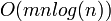$O(m n log(n))$ operation. However by saving the lists between cycles and realizing that most bodies will not have changed order too much (temporal and spatial coherence), the sort comes down to a $O(m n)$ operation.

So similar to grid methods the average case should be $O(n)$, though in practice grid methods should do a better job of culling collisions. If multiple axis are used and chosen well, I think the worst case performance becomes $O(m n log(n))$.

It is usually a good idea to choose axis that are not the x or y axis, since bodies will tend to clump along the y axis (think lots of balls sitting at the bottom of the screen) and x axis (think a vertical stack of bodies). If two axis are used, they should be orthogonal to each other. More than two I'm not sure, but probably evenly distributed on the unit circle is a good idea.

Hash sort

Sort of a combination of the grid methods and the linked list sort. Just like with the linked list sort bodies are projected against arbitrary axes. However instead of adding the results to a linked list, each axis has a hash table. Possible collisions are from hash collisions.

The primary advantage over a linked list is that the sorting is done implicitly, which eliminates a large amount of computation. The primary disadvantage over a linked list is that the universe must be finitely bounded like with grid methods.

Just like with a grids, a hierarchical hash table can be used instead of a uniform hash table. The smallest level in the hash table such that the body takes up at most two cells is chosen.